Antiferromagnetic bilayers

• in this notebook we compute the dispersion relation of two 20 nm thick permalloy layers separated with a 2 nm non-magnetic spacer

• the ferromagnetic layers are antiferromagnetically coupled via RKKY, the bilinear term of the interlayer exchange coupling

import tetrax as tx
import numpy as np
%matplotlib notebook
import matplotlib.pyplot as plt

sample = tx.create_sample(geometry="layer", name="Bilayer_iec")
sample.Msat = 800e3
sample.Aex = 13e-12
sample.J1 = -3e-4
mesh = tx.geometries.bilayer_line_trace(20,20,2,1)
sample.set_geom(mesh)

Setting geometry and calculating discretized differential operators on mesh.
Done.

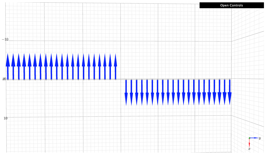
Setting initial state antiparallel

sample.mag = np.piecewise(sample.xyz, [sample.xyz.y < 0, sample.xyz.y >= 0], [[-1,0,0], [1,0,0]])
sample.show(scale = 5)

• We need to use a small field, since for k=0 the frequncy is zero for one of the branches and the eigensolver might fail to converge

exp = tx.create_experimental_setup(sample,name="thickness_20nm")
Bext = 1e-5
exp.Bext = [Bext,0,0]
dispersion = exp.eigenmodes(kmin=-40e6,kmax=40e6,Nk=201, num_modes=5,num_cpus=-1)

100%|██████████| 201/201 [00:28<00:00,  7.03it/s]

Dispersion of the acustical and optical branches

k_ = dispersion["k (rad/m)"]
plt.figure()
for i in range(2):
    plt.plot(k_*1e-6, dispersion[f"f{i} (GHz)"].values, ls="--", marker="", markersize=5, alpha=1)

plt.xlabel("Wave vector (rad/µm)")
plt.ylabel("Frequency (GHz)")
plt.xlim([-40,40])
plt.ylim([0,25])
plt.show()