tetrax.core package#
Subpackages#
Submodules#
tetrax.core.experimental_setup module#
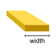
- class tetrax.core.experimental_setup.CPWAntenna(width, gap, spacing)#
Bases:
tetrax.core.experimental_setup._AbstractMicrowaveAntennaCoplanar-waveguide antenna. The antenna is assumed to be infinitely thin.
- Attributes
Methods
get_mesh
get_microwave_field_function
- get_mesh(span)#
- get_microwave_field_function(xyz)#
- class tetrax.core.experimental_setup.CurrentLoopAntenna(width, radius)#
Bases:
tetrax.core.experimental_setup._AbstractMicrowaveAntennaAntenna with the shape of a current loop.
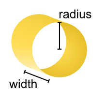
The current loop is oriented in the \(xy\) plane. For calculations, the current loop is taken to be infinitely thin in radial direction.
- Attributes
Methods
get_mesh
get_microwave_field_function
- get_mesh(span)#
- get_microwave_field_function(xyz)#
- class tetrax.core.experimental_setup.ExperimentalSetup(sample, name='my_experiment')#
Bases:
objectExperimental setup built around a
samplein which external parameters are defined and numerical experiments can be conducted.- Attributes
- sample
AbstractSample Sample object on which numerical experiments are conducted.
- name
str Name of the experimental setup, used to store results (default is
"my_experiment").- Bext
MeshVector Vector field of the static external magnetic field (given in T). Can also be set as a triplet, e.g. as
[0, 0, 0.5]for a homogeneous field of 500 mT in \(z\) direction.- antenna
_AbstractMicrowaveAntenna Microwave antenna in the experimental setup (see User Guide for details).
- sample
Methods
absorption([auto_eigenmodes, fmin, fmax, ...])Obtain the microwave absorption of the calculated eigensystem with respect to the microwave
antennain the experimental setup.eigenmodes([kmin, kmax, Nk, num_modes, k, ...])Calculate the spin-wave eigenmodes an their frequencies/dispersion of the sample in its current state using a dynamic matrix approach.
relax([tol, continue_with_least_squares, ...])Relax the magnetization
magof a sample in the experimental setup by minimizing the total magnetic energy.show([comp, scale, show_antenna])Shows the experimental setup, including external fields and microwave antennna.
- property Bext#
- absorption(auto_eigenmodes=False, fmin=0, fmax=30, Nf=200, k=None, verbose=True)#
Obtain the microwave absorption of the calculated eigensystem with respect to the microwave
antennain the experimental setup.- Parameters
- auto_eigenmodesbool
If no eigenmodes are available in this experimental setup, calculate eigenmodes with default settings.
- fmin
float Minimum microwave frequency in GHz for which the absorption line is calculated (default is 0).
- fmax
float Maximum microwave frequency in GHz for which the absorption line is calculated (default is 30).
- Nf
int Number of microwave frequencies for which the absorption is calculated (default is 200).
- k
float If set to a value, the absorption line is calculated only for a single wave vector (default is
None). Also, the full dynamic susceptibility is saved to a dataframe. This argument is ignored in confined samples.- verbosebool
Output progress of the calculation (default is
True).
- Returns
- susceptibility
pandas.DataFrame Only if
kis notNoneor sample is a confined sample. Contains frequency-dependent real and imaginary part as well as magnitude as phase and magnitude of the averaged dynamic susceptiblity.- (absorbed_power, wave_vectors, frequencies)(
numpy.ndarray,numpy.ndarray,numpy.ndarray) If
kisNoneand sample is a waveguide or a layer sample. Saves the wave-vector and frequency- dependent microwave-power absorption (absorbed_power) together with the corresponding wave vectors and frequencies as a 2D arrays.
- susceptibility
Notes
The return of a wave-vector-dependent absorption calculation can be plotted using matplotlib as
>>> absorbed_power, wave_vectors, frequencies = exp.absorption(...)
>>> import matplotlib.pyplot as plt
>>> plt.pcolormesh(wave_vectors, frequencies, absorbed_power)
References
- 1
Verba, et al., “Damping of linear spin-wave modes in magnetic nanostructures: Local, nonlocal, and coordinate-dependent damping”, Phys. Rev. B 98, 104408 (2018)
- 2
Körber, et al., “Symmetry and curvature effects on spin waves in vortex-state hexagonal nanotubes”, Phys. Rev. B 104, 184429 (2021)
Examples
- property antenna#
- eigenmodes(kmin=- 40000000.0, kmax=40000000.0, Nk=81, num_modes=20, k=None, no_dip=False, h0_dip=False, num_cpus=1, save_modes=True, save_local=False, save_magphase=False, perturbed_dispersion=False, save_stiffness_fields=False, verbose=True)#
Calculate the spin-wave eigenmodes an their frequencies/dispersion of the sample in its current state using a dynamic matrix approach.
The eigensystem is calculuated by numerically solving the linearized equation of motion of magnetizion (see User Guide for details). For waveguides or layer samples, a finite-element propagating-wave dynamic-matrix approach is used [1]. The dispersion is returned as a
pandas.DataFrame. Additionally, it is saved asdispersion.csv(ordispersion_perturbedmodes.csv, ifperturbed_dispersion=True) in the folder of the experimental setup.- Parameters
- kmin
float Minimum wave vector in rad/m (default is -40e6). This argument is ignored when calculating the eigensystem for confined samples.
- kmax
float Maximum wave vector in rad/m (default is 40e6). This argument is ignored when calculating the eigensystem for confined samples.
- Nk
int Number of wave-vector values, for which the mode frequencies are calculated. This argument is ignored when calculating the eigensystem for confined samples (default is 81).
- num_modes
int Determines how many modes (for confined samples) or branches of the dispersion (for waveguides and layers samples) are calculated in total (default is 20).
- k
float If set to a
floatvalue, the eigensystem is only calculated for a single wave vector (default isNone). This argument is ignored when calculating the eigensystem for confined samples.- no_dipbool
Exclude dipolar interaction from calculations (default is
False).- h0_dipbool
If
no_dipisTrue, still retain dipolar contributions in the equilibrium effective field.- num_cpus
int Number of CPU cores to be used in parallel for calculations (default is 1). If set to
-1, all available cores are used.- save_modesbool
Saves real and imaginary part of the mode profiles in cartesian basis as vtk files (default is
True). The mode profiles are saved in a/mode-profilessubdirectory in the folder of the experimental setup.- save_localbool
If
save_modesis alsoTrue, save the components of the mode profiles in the basis locally orthogonal to the equilibrum magnitization (default isFalse). The local components are saved in the samevtkfile as cartesian components.- save_magphase
If
save_modesis alsoTrue, save magnetide and phase of the mode-profile components (default isFalse). Saved in the same- perturbed_dispersionbool
After calculating the eigenmodes/normalmodes (possibly with
no_dip=True), calculate the zeroth-order pertubation of the dispersion including dynamic dipolar fields according to Ref [2]. Gives approximation for dispersion without dipolar hybridization (default isFalse). The results are appended to the returneddispersiondataframe.- save_stiffness_fieldsbool
If perturbed_dispersion is also
True, append the unitless individual stiffness fields (components) within the perturbed dispersion to thedispersiondataframe (default isFalse). Allows to numerically reverse engineer general spin-wave dispersions [2].- verbosebool
Output progress of the calculation (default is
True).
- kmin
- Returns
- dispersion
pandas.DataFrame Dataframe (table) containing the calculated dispersion.
- dispersion
Notes
By default, the
dispersionDataFrame is structured ask (rad/m)
f0 (GHz)
f1 (GHz)
…
-40e6
1.426
2.352
…
…
…
…
…
In case
perturbed_dispersion=True, additional columns are added ask (rad/m)
f0 (GHz)
f_pert_0 (GHz)
…
-40e6
1.426
484
…
…
…
…
…
Additionally, if
save_stiffnessfields=True, the unitless stiffness fields per magnetic interaction are also appendedk (rad/m)
f0 (GHz)
f_pert_0 (GHz)
Re(N21_exc)_0
…
-40e6
1.426
484
0.431
…
…
…
…
…
…
Indivual columns/rows can be obtained in the usual way for pandas.DataFrame`, for example, with
>>> k = dispersion["k (rad/m)"]
>>> first_row = dispersion.iloc[0]
References
- 1
Körber, et al., “Finite-element dynamic-matrix approach for spin-wave dispersions in magnonic waveguides with arbitrary cross section”, AIP Advances 11, 095006 (2021)
- 2(1,2)
Körber and Kákay, “Numerical reverse engineering of general spin-wave dispersions: Bridge between numerics and analytics using a dynamic-matrix approach”, Phys. Rev. B 104, 174414 (2021)
Examples
- relax(tol=1e-12, continue_with_least_squares=False, return_last=False, save_mag=True, fname='mag.vtk', verbose=True)#
Relax the magnetization
magof a sample in the experimental setup by minimizing the total magnetic energy.- Parameters
- tol
float, optional Tolerance at which the minimization is considered successful (default is
1e-12).- continue_with_least_squaresbool
If minimization with conjugate-gradient method was not successful, continue with least-squares method (default is
False). This is more stable, but slower.- return_lastbool
If minimization was not successful, set the last iteration step as the sample magnetization (default is
False).- save_magbool
Save the resulting magnetization as vtk file to the folder of the experimental setup (default is
True).- fname
str Filename for magnetization file (default is
mag.vtk).- verbosebool
Output progress of the calculation (default is
True).
- tol
- Returns
- successbool
If the relaxation was successful of not.
Notes
For waveguide samples, the equilibration is not totally stable yet. Please use with care and check the resulting equilibrium states.
Examples
- show(comp='vec', scale=5, show_antenna=True)#
Shows the experimental setup, including external fields and microwave antennna.
- class tetrax.core.experimental_setup.HomogeneousAntenna(theta=0, phi=0)#
Bases:
tetrax.core.experimental_setup._AbstractMicrowaveAntennaAntenna which produces a homogeneous microwave field.
- Attributes
Methods
get_mesh
get_microwave_field_function
- get_mesh()#
- get_microwave_field_function(xyz)#
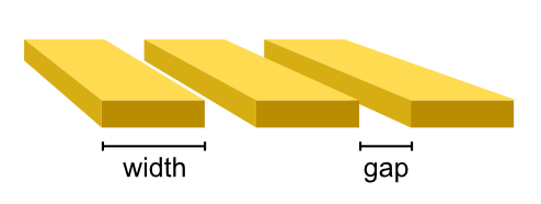
- class tetrax.core.experimental_setup.StriplineAntenna(width, spacing)#
Bases:
tetrax.core.experimental_setup._AbstractMicrowaveAntennaStripline antenna. The antenna is assumed to be infinitely thin.
- Attributes
Methods
get_mesh
get_microwave_field_function
- get_mesh(span)#
- get_microwave_field_function(xyz)#
- tetrax.core.experimental_setup.create_experimental_setup(sample, name: str = 'my_experiment') tetrax.core.experimental_setup.ExperimentalSetup#
Creates an experimental setup around a given sample.
- Parameters
- sample
AbstractSample Sample object to create ExperimentalSetup around.
- name
str Name of the experimental setup.
- sample
- Returns
tetrax.core.mesh module#
This core submodule provides several subclasses of np.ndarray to define different scalar and vector fields on meshes. The import convention
>>> import numpy as np
is used.
- class tetrax.core.mesh.FlattenedAFMMeshVector(input_array)#
Bases:
numpy.ndarrayClass of shape for antiferromagnets (6*nx,) to hold the flattened vector fields of each sublattice defined on the same mesh.
The entries of the vector are ordered according to
\[\mathbf{a} = (a_{x_1}, ... , a_{x_N}, a_{y_1}, ... , a_{y_N}, a_{z_1}, ... , a_{z_N}, b_{x_1}, ... , b_{x_N}, b_{y_1}, ... , b_{y_N}, b_{z_1}, ... , b_{z_N})\]while \(N\) = nx and \(\mathbf{a}\), \(\mathbf{b}\) are the vector fields of the respective sublattices. The input array_like needs to be one dimensional. The number of nodes nx is inferred from the input array.
See also
- Attributes
- nx
int Number of nodes.
- x1
MeshScalar The \(x\) component of the first sublattice vector field at each mesh node.
- y1
MeshScalar The \(y\) component of the first sublattice vector field at each mesh node.
- z1
MeshScalar The \(z\) component of the first sublattice vector field at each mesh node.
- x2
MeshScalar The \(x\) component of the second sublattice vector field at each mesh node.
- y2
MeshScalar The \(y\) component of the second sublattice vector field at each mesh node.
- z2
MeshScalar The \(z\) component of the second sublattice vector field at each mesh node.
- nx
Methods
to_two_unflattened()
Returns the indivudal vector fields of the sublattices as two separate :py:class:`MeshVector`s.
- to_two_unflattened()#
- property x1#
- property x2#
- property y1#
- property y2#
- property z1#
- property z2#
- class tetrax.core.mesh.FlattenedLocalMeshVector(input_array)#
Bases:
numpy.ndarrayClass for two-component vector fields of shape (2*nx,) defined on a mesh.
This class is used to describe vector fields locally ortoghonal and expressed in the \((u,v,w)\) basis attached to the equilibrium magnetization, hence the name. Because of that, the third (\(w\)) compontent of the vector field is always zero and therefore omitted. The entries of the vector field are ordered according to
\[\mathbf{a} = (a_{u_1}, ... , a_{u_N}, a_{v_1}, ... , a_{v_N})\]while \(N\) = nx. The input array_like needs to be two dimensional with shape[1] = 2 (array of triplets). The number of nodes nx is inferred from shape[0] of the input array.
- Attributes
- nx
int Number of nodes.
- u
MeshScalar The first (\(u\)) component of the vector field at each mesh node.
- v
MeshScalar The second (\(v\)) component of the vector field at each mesh node.
- nx
Methods
to_unflattened()
Returns the vector field as an unflattened
LocalMeshVector.- to_unflattened()#
- property u#
- property v#
- class tetrax.core.mesh.FlattenedMeshVector(input_array)#
Bases:
numpy.ndarrayClass for three-component vector fields of shape (3*nx,) defined on a mesh.
The entries of the vector are ordered according to
\[\mathbf{a} = (a_{x_1}, ... , a_{x_N}, a_{y_1}, ... , a_{y_N}, a_{z_1}, ... , a_{z_N})\]while \(N\) = nx. The input array_like needs to be one dimensional and cannot be a
FlattenedLocalMeshVector. The number of nodes nx is inferred from the length of the input array.See also
- Attributes
- nx
int Number of nodes.
- x
MeshScalar The \(x\) component of the vector field at each mesh node.
- y
MeshScalar The \(y\) component of the vector field at each mesh node.
- z
MeshScalar The \(z\) component of the vector field at each mesh node.
- nx
Methods
to_ùnflattened()
Returns the vector field as an unflattened
MeshVector.- to_unflattened()#
- property x#
- property y#
- property z#
- class tetrax.core.mesh.LocalMeshVector(input_array)#
Bases:
numpy.ndarrayClass for two-component vector fields of shape (nx, 2) defined on a mesh.
This class is used to describe vector fields locally ortoghonal and expressed in the \((u,v,w)\) basis attached to the equilibrium magnetization, hence the name. Because of that, the third (\(w\)) compontent of the vector field is always zero and therefore omitted. The entries of the vector field are ordered according to
\[\begin{split}\mathbf{a} = \begin{pmatrix} a_{u_1} & a_{v_1} \\ & \vdots & \\ a_{u_N} & a_{v_N} \\ \end{pmatrix}\end{split}\]while \(N\) = nx. The input array_like needs to be one dimensional and cannot be a
FlattenedMeshVector. The number of nodes nx is inferred from the length of the input array.See also
- Attributes
- nx
int Number of nodes.
- u
MeshScalar The first (\(u\)) component of the vector field at each mesh node.
- v
MeshScalar The second (\(v\)) component of the vector field at each mesh node.
- nx
Methods
to_flattened()
Returns the vector field as a
FlattenedLocalMeshVector.- to_flattened()#
- property u#
- property v#
- class tetrax.core.mesh.MeshScalar(input_array)#
Bases:
numpy.ndarrayClass for scalar fields defined on a mesh.
Input array_like needs to be one dimensional. The number of nodes nx is inferred from the length of the input array.
- Attributes
- nx
int Number of nodes.
- nx
Methods
all([axis, out, keepdims, where])Returns True if all elements evaluate to True.
any([axis, out, keepdims, where])Returns True if any of the elements of a evaluate to True.
argmax([axis, out, keepdims])Return indices of the maximum values along the given axis.
argmin([axis, out, keepdims])Return indices of the minimum values along the given axis.
argpartition(kth[, axis, kind, order])Returns the indices that would partition this array.
argsort([axis, kind, order])Returns the indices that would sort this array.
astype(dtype[, order, casting, subok, copy])Copy of the array, cast to a specified type.
byteswap([inplace])Swap the bytes of the array elements
choose(choices[, out, mode])Use an index array to construct a new array from a set of choices.
clip([min, max, out])Return an array whose values are limited to
[min, max].compress(condition[, axis, out])Return selected slices of this array along given axis.
conj()Complex-conjugate all elements.
conjugate()Return the complex conjugate, element-wise.
copy([order])Return a copy of the array.
cumprod([axis, dtype, out])Return the cumulative product of the elements along the given axis.
cumsum([axis, dtype, out])Return the cumulative sum of the elements along the given axis.
diagonal([offset, axis1, axis2])Return specified diagonals.
dump(file)Dump a pickle of the array to the specified file.
dumps()Returns the pickle of the array as a string.
fill(value)Fill the array with a scalar value.
flatten([order])Return a copy of the array collapsed into one dimension.
getfield(dtype[, offset])Returns a field of the given array as a certain type.
item(*args)Copy an element of an array to a standard Python scalar and return it.
itemset(*args)Insert scalar into an array (scalar is cast to array's dtype, if possible)
max([axis, out, keepdims, initial, where])Return the maximum along a given axis.
mean([axis, dtype, out, keepdims, where])Returns the average of the array elements along given axis.
min([axis, out, keepdims, initial, where])Return the minimum along a given axis.
newbyteorder([new_order])Return the array with the same data viewed with a different byte order.
nonzero()Return the indices of the elements that are non-zero.
partition(kth[, axis, kind, order])Rearranges the elements in the array in such a way that the value of the element in kth position is in the position it would be in a sorted array.
prod([axis, dtype, out, keepdims, initial, ...])Return the product of the array elements over the given axis
ptp([axis, out, keepdims])Peak to peak (maximum - minimum) value along a given axis.
put(indices, values[, mode])Set
a.flat[n] = values[n]for all n in indices.ravel([order])Return a flattened array.
repeat(repeats[, axis])Repeat elements of an array.
reshape(shape[, order])Returns an array containing the same data with a new shape.
resize(new_shape[, refcheck])Change shape and size of array in-place.
round([decimals, out])Return a with each element rounded to the given number of decimals.
searchsorted(v[, side, sorter])Find indices where elements of v should be inserted in a to maintain order.
setfield(val, dtype[, offset])Put a value into a specified place in a field defined by a data-type.
setflags([write, align, uic])Set array flags WRITEABLE, ALIGNED, WRITEBACKIFCOPY, respectively.
sort([axis, kind, order])Sort an array in-place.
squeeze([axis])Remove axes of length one from a.
std([axis, dtype, out, ddof, keepdims, where])Returns the standard deviation of the array elements along given axis.
sum([axis, dtype, out, keepdims, initial, where])Return the sum of the array elements over the given axis.
swapaxes(axis1, axis2)Return a view of the array with axis1 and axis2 interchanged.
take(indices[, axis, out, mode])Return an array formed from the elements of a at the given indices.
tobytes([order])Construct Python bytes containing the raw data bytes in the array.
tofile(fid[, sep, format])Write array to a file as text or binary (default).
tolist()Return the array as an
a.ndim-levels deep nested list of Python scalars.tostring([order])A compatibility alias for tobytes, with exactly the same behavior.
trace([offset, axis1, axis2, dtype, out])Return the sum along diagonals of the array.
transpose(*axes)Returns a view of the array with axes transposed.
var([axis, dtype, out, ddof, keepdims, where])Returns the variance of the array elements, along given axis.
view([dtype][, type])New view of array with the same data.
dot
- class tetrax.core.mesh.MeshVector(input_array)#
Bases:
numpy.ndarrayClass for three-component vector fields of shape (nx, 3) defined on a mesh.
The entries of the vector are ordered according to
\[\begin{split}\mathbf{a} = \begin{pmatrix} a_{x_1} & a_{y_1} & a_{z_1} \\ & \vdots & \\ a_{x_N} & a_{y_N} & a_{z_N} \\ \end{pmatrix}\end{split}\]while \(N\) = nx. The input array_like needs to be two dimensional with shape[1] = 3 (array of triplets). The number of nodes nx is inferred from shape[0] of the input array.
- Attributes
- nx
int Number of nodes.
- x
MeshScalar The \(x\) component of the vector field at each mesh node.
- y
MeshScalar The \(y\) component of the vector field at each mesh node.
- z
MeshScalar The \(z\) component of the vector field at each mesh node.
- nx
Methods
to_flattened()
Returns the vector field as
FlattenedMeshVector.- to_flattened()#
- property x#
- property y#
- property z#
- tetrax.core.mesh.make_flattened_AFM(a, b)#
Creates a
FlattenedAFMMeshVectorfrom two individual :py:class:`MeshVector`s.- Parameters
- a
MeshVector Vector field of the first sublattice.
- b
MeshVector Vector field of the second sublattice.
- a
- Returns
FlattenedAFMMeshVectorFlattened vector field of the AFM lattice.
See also
tetrax.core.operators module#
- class tetrax.core.operators.BulkDMIOperator(*args, **kwargs)#
Bases:
scipy.sparse.linalg._interface.LinearOperator- Attributes
HHermitian adjoint.
TTranspose this linear operator.
Methods
__call__(x)Call self as a function.
adjoint()Hermitian adjoint.
dot(x)Matrix-matrix or matrix-vector multiplication.
matmat(X)Matrix-matrix multiplication.
matvec(x)Matrix-vector multiplication.
rmatmat(X)Adjoint matrix-matrix multiplication.
rmatvec(x)Adjoint matrix-vector multiplication.
transpose()Transpose this linear operator.
set_k
- set_k(k)#
- class tetrax.core.operators.CubicAnisotropyLinearOperator(*args, **kwargs)#
Bases:
scipy.sparse.linalg._interface.LinearOperator- Attributes
HHermitian adjoint.
TTranspose this linear operator.
Methods
__call__(x)Call self as a function.
adjoint()Hermitian adjoint.
dot(x)Matrix-matrix or matrix-vector multiplication.
matmat(X)Matrix-matrix multiplication.
matvec(x)Matrix-vector multiplication.
nonlinear_field(vec)Full nonlinear anistropy.
nonlinear_field_old(vec)Full nonlinear anistropy.
rmatmat(X)Adjoint matrix-matrix multiplication.
rmatvec(x)Adjoint matrix-vector multiplication.
set_new_param(conf, nx)Set new parameters for unixial anisotropy.
transpose()Transpose this linear operator.
make_sparse_mat_with_current_m0
- make_sparse_mat_with_current_m0()#
- nonlinear_field(vec)#
Full nonlinear anistropy. Returns the cubic anisotropy field of a given vector. This is not a linear operator.
- nonlinear_field_old(vec)#
Full nonlinear anistropy. Returns the cubic anisotropy field of a given vector. This is not a linear operator.
- set_new_param(conf, nx)#
Set new parameters for unixial anisotropy.
- class tetrax.core.operators.DipolarOperator(*args, **kwargs)#
Bases:
scipy.sparse.linalg._interface.LinearOperator- Attributes
HHermitian adjoint.
TTranspose this linear operator.
Methods
__call__(x)Call self as a function.
adjoint()Hermitian adjoint.
dot(x)Matrix-matrix or matrix-vector multiplication.
matmat(X)Matrix-matrix multiplication.
matvec(x)Matrix-vector multiplication.
rmatmat(X)Adjoint matrix-matrix multiplication.
rmatvec(x)Adjoint matrix-vector multiplication.
transpose()Transpose this linear operator.
set_k
- set_k(k)#
- class tetrax.core.operators.ExchangeOperator(*args, **kwargs)#
Bases:
scipy.sparse.linalg._interface.LinearOperator- Attributes
HHermitian adjoint.
TTranspose this linear operator.
Methods
__call__(x)Call self as a function.
adjoint()Hermitian adjoint.
dot(x)Matrix-matrix or matrix-vector multiplication.
matmat(X)Matrix-matrix multiplication.
matvec(x)Matrix-vector multiplication.
rmatmat(X)Adjoint matrix-matrix multiplication.
rmatvec(x)Adjoint matrix-vector multiplication.
transpose()Transpose this linear operator.
set_k
- set_k(k)#
- class tetrax.core.operators.InterfacialDMIOperator(*args, **kwargs)#
Bases:
scipy.sparse.linalg._interface.LinearOperator- Attributes
HHermitian adjoint.
TTranspose this linear operator.
Methods
__call__(x)Call self as a function.
adjoint()Hermitian adjoint.
dot(x)Matrix-matrix or matrix-vector multiplication.
matmat(X)Matrix-matrix multiplication.
matvec(x)Matrix-vector multiplication.
rmatmat(X)Adjoint matrix-matrix multiplication.
rmatvec(x)Adjoint matrix-vector multiplication.
transpose()Transpose this linear operator.
set_k
- set_k(k)#
- class tetrax.core.operators.InvTotalDynMat(*args, **kwargs)#
Bases:
scipy.sparse.linalg._interface.LinearOperatorInverse of Dynamic Matrix
- Attributes
HHermitian adjoint.
TTranspose this linear operator.
Methods
__call__(x)Call self as a function.
adjoint()Hermitian adjoint.
dot(x)Matrix-matrix or matrix-vector multiplication.
matmat(X)Matrix-matrix multiplication.
matvec(x)Matrix-vector multiplication.
rmatmat(X)Adjoint matrix-matrix multiplication.
rmatvec(x)Adjoint matrix-vector multiplication.
transpose()Transpose this linear operator.
- exception tetrax.core.operators.InvertError(k, after_iter, already_sucess, message)#
Bases:
tetrax.core.operators.ErrorException raised for errors in inversion of total dynamic matrix.
- tetrax.core.operators.N_dip(m, k, ksquared_mat_a_n, ksquared_mat_a_nb, nx, div_x, div_y, poiss, boundary_nodes, dense, laplace, grad_x, grad_y, a_n)#
- class tetrax.core.operators.SuperLUInv(*args, **kwargs)#
Bases:
scipy.sparse.linalg._interface.LinearOperatorSuperLU object as LinearOperator
- Attributes
HHermitian adjoint.
TTranspose this linear operator.
Methods
__call__(x)Call self as a function.
adjoint()Hermitian adjoint.
dot(x)Matrix-matrix or matrix-vector multiplication.
matmat(X)Matrix-matrix multiplication.
matvec(x)Matrix-vector multiplication.
rmatmat(X)Adjoint matrix-matrix multiplication.
rmatvec(x)Adjoint matrix-vector multiplication.
transpose()Transpose this linear operator.
- class tetrax.core.operators.TotalDynMat(*args, **kwargs)#
Bases:
scipy.sparse.linalg._interface.LinearOperator- Attributes
HHermitian adjoint.
TTranspose this linear operator.
Methods
__call__(x)Call self as a function.
adjoint()Hermitian adjoint.
dot(x)Matrix-matrix or matrix-vector multiplication.
matmat(X)Matrix-matrix multiplication.
matvec(x)Matrix-vector multiplication.
rmatmat(X)Adjoint matrix-matrix multiplication.
rmatvec(x)Adjoint matrix-vector multiplication.
transpose()Transpose this linear operator.
set_k
- set_k(k, sparse_mat_k)#
- class tetrax.core.operators.UniAxialAnisotropyOperator(*args, **kwargs)#
Bases:
scipy.sparse.linalg._interface.LinearOperator- Attributes
HHermitian adjoint.
TTranspose this linear operator.
Methods
__call__(x)Call self as a function.
adjoint()Hermitian adjoint.
dot(x)Matrix-matrix or matrix-vector multiplication.
matmat(X)Matrix-matrix multiplication.
matvec(x)Matrix-vector multiplication.
rmatmat(X)Adjoint matrix-matrix multiplication.
rmatvec(x)Adjoint matrix-vector multiplication.
transpose()Transpose this linear operator.
make_sparse_mat
- make_sparse_mat()#
- tetrax.core.operators.cross_operator(nx)#
Return the rotated cross product operator as a crs_matrix.
tetrax.core.sample module#
- class tetrax.core.sample.AbstractSample(name, geometry, magnetic_order, dim)#
Bases:
abc.ABCBase class for the concrete sample classes
_ConfinedSampleFM_ConfinedSampleAFM_WaveguideSampleFM_WaveguideSampleAFM_LayerSampleFM_LayerSampleAFM
which are created by multiple-inheritance from this base class together with mixin classes for magnetic order (FM or AFM) and geometry type (confined, waveguide, layer). The available attributes for material parameters depend on the magnetic order (see User Guide for details).
- Attributes
- name
str Name of the sample.
- nx
int Total number of nodes in the mesh of the sample.
- nb
int Number of boundary nodes in the mesh of the sample.
- mesh
meshio.Mesh Mesh of the sample.
- xyz
MeshVector Coordinates on the mesh of the sample.
- scale
float Scale of the sample (default is 1e-9, such that all spatial dimensions are given in nanometer).
- name
Methods
field_to_file(field[, fname, qname])Calls the
tetrax.helpers.io.write_field_to_file()function to write scalar- or vector field to a file.plot(fields[, comp, scale, labels])Plot a vector or scalar field which is defined on each node of the mesh.
read_mesh(fname)Read a mesh from a file using meshio and set it as the geometry of a sample.
set_geom(mesh)Set the geometry/mesh of the sample and do neccesary preprocessing for later calculations.
show([show_node_labels, show_mag, comp, scale])Show the sample.
- field_to_file(field, fname='field.vtk', qname=None)#
Calls the
tetrax.helpers.io.write_field_to_file()function to write scalar- or vector field to a file.
- plot(fields, comp='vec', scale=5, labels=None)#
Plot a vector or scalar field which is defined on each node of the mesh. Multiple fields can be plotted at the same time.
- Parameters
- fields
numpy.arrayorlist(numpy.array) Scalar field of shape (nx,), vector field of shape (nx,3) or list containing any choice of the aforementioned.
- comp{“vec”, “x”, “y”, “z”}
If field is a vector field, this parameter determines which component will be plotted.
- scale
float Determines the scale of the vector glyphs used to visualize a vectorfield (default is 5).
- labels
strorlist(str) Label(s) of the vectorfield(s) to be plotted. If
labelsis a list, it needs to have the same length asfields(default isNone).
- fields
- read_mesh(fname)#
Read a mesh from a file using meshio and set it as the geometry of a sample.
- Parameters
- fname
str Name of the mesh file.
- fname
- set_geom(mesh)#
Set the geometry/mesh of the sample and do neccesary preprocessing for later calculations.
According to the dimension of the sample, the mesh is checked for compatibility. After sucessefully setting the mesh and extrancting necessary information, such as the number of nodes
nx, the coordinates of the mesh verticesxyzor the normal vectorsnv, the discretized differential operators (poisson,div_x, …) are calculated and the magnetic tensors are set up.- Parameters
- mesh
meshio.Mesh
- mesh
- abstract show(show_node_labels=False, show_mag=True, comp='vec', scale=5)#
Show the sample. Displays the mesh and, if available, the magnetization(s).
- Parameters
- show_node_labelsbool
If true, shows the label associated to each node.
- show_magbool
Show the magnetization (or magnetizations, in the case of antiferromagnetic samples).
- comp{“vec”, “x”, “y”, “z”}
Determines which component will be plotted.
- scale
float Determines the scale of the vector glyphs used to visualize the magnetization (default is 5).
- Returns
- tetrax.core.sample.create_sample(name='my_sample', geometry='waveguide', magnetic_order='FM')#
Create a sample with certain geometry and magnetic order.
- Parameters
- Returns
- sample
AbstractSample
- sample