3. Creating and defining a sample

3.1. The sample object

3.1.1. Initialization

The central object in a TetraX workflow is the sample, represented by an instance of the AbstractSample class. Much like physical samples, they are characterized by a geometry, a set of material parameters, a magnetization state and the involved magnetic interactions. In numerical experiments, the sample is additionally characterized by an underlying mesh, a scale, a set of differential operators (gradient, divergence, etc.) tied to the mesh and a number of other attributes neccessary for computation. We can create a sample using

>>> sample = tx.create_sample("name of my sample")

This will initialize a sample (without a geometry yet) with a set of default material parameters. These parameters can be accessed and set in the usual pythonic way

>>> sample.Msat = 800e3
>>> print(sample.Msat)
800.0e3

>>> print(sample.name)
"name of my sample"

The name of the sample is set purely for the purpose of storing data in a meaningful way, as all data obtained in numerical experiments is saved in a directory named after the sample.

3.1.2. Setting a geometry

Before proceeding with anything further, a specific geometry for the sample needs to be set. This is done by supplying a mesh (in meshio format) to the sample using

>>> sample.set_geom(mesh)

In the tetrax.geometries submodule, we supply a couple of templates to generate common meshes, such as cuboids, prisms, tubes, wires, and so forth. However, desired meshes can be generated also using pygmsh or even any external software, as long as the generated mesh files are readable by meshio. Mesh files can be read in using

>>> sample.read_mesh(filename)

When setting a mesh/geometry, under the hood, certain preprocessing necessary for later computations is performed. For example, the differential operators on the mesh or the normal vector field of the sample are calculated. After these calculations have been performed, important numerical parameters of the mesh can be accessed, including

• mesh, the mesh itself in meshio format,

• nx, the total number of nodes in the mesh,

• nb, the number of boundary nodes in the mesh, and

• xyz, the coordinates at each node as a MeshVector. These coordinates are expressed in units of

• scale, the characteristic length of the sample. The default is 1e-9 which means that the coordinates on the mesh are given in nanometers.

Note

The mesh of the sample can visualized using the show method on the sample, to allow for checking if the mesh was created/obtained according to the request or mesh in mind:

>>> sample.show()

3.1.3. Magnetization vector field

Once a mesh has been assigned to the sample, the magnetization vector field of the sample (mag) can be set for example as

>>> sample.mag = [0, 0, 1]

Note

A magnetization vector field can only be set for samples which already have a mesh.

In antiferromagnetic cases, the sample has a magnetization vector field for each sublattice, mag1 and mag2. To initialize an inhomogeneous magnetization, an array of shape (nx, 3) needs to supplied which can be seen as a list of triplets with each triplet representing the vector at a specific node. For convenience, a couple of template vector fields (such as domain walls, vortices, etc.) can be found in the tetrax.vectorfields submodule. These fields can be called by supplying xyz, the coordinates on the mesh.

>>> sample.mag = tx.vectorfields.bloch_wall(sample.xyz, ...)

When setting a magnetization field, the input field is automatically normalized and internally converted to a MeshVector, which is a data structure that allows to easily access the different components of the magnetization.

>>> sample.mag.x
MeshScalar([0.0, 0.0, 0.12, 0.15, ...])

Here, we see that the individual components of a mesh vector are MeshScalars, another basic data structure in TetraX. We can easily calculate the averages of these objects using the sample_average function from the tetrax.helpers.math module, which takes some vector- or scalar field and the sample itself as an input.

>>> m = tx.sample_average(sample.mag, sample)
>>> m
[0.98, 0.02, 0.0]

>>> mx = tx.sample_average(sample.mag.x, sample)
>>> mx
0.98

Note

The reason, why sample_average is not called volume_average is because not all samples have to be three-dimensional. For example, in waveguide samples, sample_average calculates the average in a cross section.

The mesh and the current magnetization of a sample (if available) can always be visualized using the show method.

>>> sample.show()

For further details, see Visualization.

3.2. Different types of samples

Depending on the specific type of geometry and magnetic order, concrete subclasses of AbstractSample can be generated which are distinguished by their set of possible material parameters (ferromagnetic or antiferromagnetic), dimensionality, or numerical solvers needed to calculate magnetization dynamics or statics. The type of sample is chosen when creating the sample. At the beginning of this section, a sample was created by calling tetrax.create_sample(). Per default, this function creates a ferromagnetic waveguide sample. However, different options are possible.

tetrax.core.sample.create_sample(name='my_sample', geometry='waveguide', magnetic_order='FM')

Create a sample with certain geometry and magnetic order.

Parameters

geometrystr, {“confined”, “waveguide”, “layer”}

Geometry of the sample (default is “waveguide”).

magnetic_orderstr {“FM”, “AFM”}, optional

Magnetic order of the material. Can be either ferromagnetic (“FM”) or antiferromagnetic (“AFM”). The default is “FM”.

Returns

sampleAbstractSample

We can see from the geometry parameter, that different types of samples can be selected:

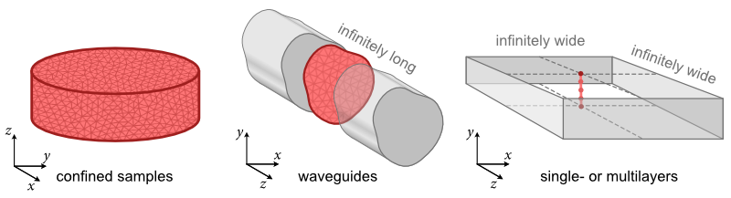
• confined samples such as disks, cuboids, spheres or Möbius ribbons. These types of samples are often the subject of standard three-dimensional micromagnetic simulations. Only in such samples, an LLG solver can be used. Using a confined-wave dynamic-matrix approach, the normal modes of confined samples can be calculated.

• waveguide samples are infinitely long in one direction (here, the \(z\) direction). Moreover, their (equilibrium) magnetization is taken to be translationally invariant in this direction. Such samples are modelled by discretizing only a single cross section of the waveguide. A propagating-wave dynamic-matrix approach can be used to calculate the normal modes as a function of the wave vector \(k\) along the \(z\) direction.

• layer samples consist of one or multiple infinetely extended layers which are modelled by discretizing a line trace along the thickness of the layer(s). The (equilibrium) magnetization is taken to be homogeneous within the layer planes. A propagating-wave dynamic-matrix approach can be used to calculate the normal modes as a function of the wave vector \(k\) along the \(z\) direction.

For all three different types of samples, energy minimizers are implemented to calculated the magnetic ground states.

Warning

At the moment, only ferromagnetic waveguide samples are fully supported.

3.3. Specific geometries

Template geometries (mesh generators) are all available in the tetrax.geometries module. Even though they are implemented in submodules, all of them can be accessed in the namespace of tetrax.geometries. For examples

sample.set_geom(tx.geometries.tube_cross_section(r=20, R=30, lc=3))

Note

For a given sample, only such meshes can be set which fit the type of the sample selected. For example, it is not possible to set a three-dimensional cuboid mesh for a sample which represents the cross section of an infinitely long waveguide.

3.3.1. Geometries for confined samples

To be implemented.

3.3.2. Geometries for waveguide samples

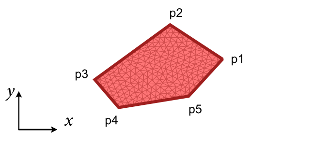
tetrax.geometries.geometries2D.polygonal_cross_section(points, lc=5)

Creates a mesh with the cross section of a polygonal wire.

Parameters

pointslist (Point)

List of points defining the corners of the polygon.

lcfloat

Characteristic length of mesh (default is 5).

Returns

meshmeshio.Mesh

See also

round_wire_cross_section, rectangle_cross_section

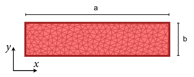
tetrax.geometries.geometries2D.rectangle_cross_section(a, b, lca=5, lcb=5)

Creates a regular mesh with rectangular cross section.

Parameters

afloat

Width of the rectangle.

bfloat

Thickness of the rectangle.

lcafloat

characteristic mesh length along the width (Default is 5). The number of FEM layers along the width will be a/lca + 1.

lcbfloat

characteristic mesh length along the thickness (Default is 5). The number of FEM layers along the thickness will be b/lcb + 1.

Returns

meshmeshio.Mesh

See also

round_wire_cross_section, polygonal_cross_section

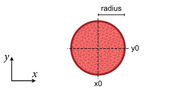
tetrax.geometries.geometries2D.round_wire_cross_section(R, lc=5, x0=0, y0=0)

Creates a mesh with the cross section of a round wire.

Parameters

Rfloat

Radius of the round wire.

lcfloat

Characteristic length of mesh (default is 5).

x0float

x coordinate of the origin (Default is 0).

y0float

y coordinate of the origin (Default is 0).

Returns

meshmeshio.Mesh

See also

polygonal_cross_section, rectangle_cross_section

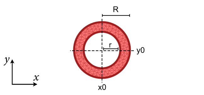
tetrax.geometries.geometries2D.tube_cross_section(r, R, lc=5, x0=0, y0=0)

Creates a mesh with the cross section of a tube.

Parameters

rfloat

Inner radius of the tube.

Rfloat

Outer radius of the tube.

lcfloat

Characteristic length of mesh (default is 5).

x0float

x coordinate of the origin (Default is 0).

y0float

y coordinate of the origin (Default is 0).

Returns

meshmeshio.Mesh

See also

tube_segment_cross_section, round_wire_cross_section, polygonal_cross_section

tetrax.geometries.geometries2D.tube_segment_cross_section(arc_length, thickness, angle, lc=5, shifted_to_origin=True)

Creates a mesh with the cross section of a tube segment.

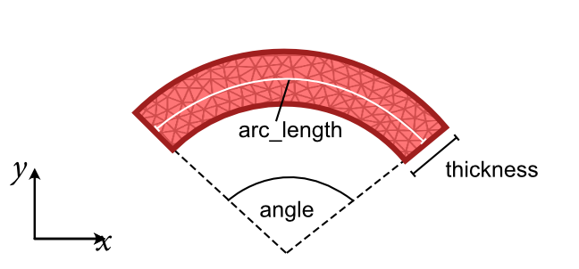
Parameters

arc_lengthfloat

Average arc length of the tube segment (at the center surface).

thicknessfloat

Thickness of the tube segment.

anglefloat

Opening angle of the tube segment (degrees).

lcfloat

Characteristic length of mesh (default is 5).

shifted_to_originbool

If True, shift the tube segment to the coordinate origin (default is True). Otherwise, the origin will be the symmetry axis of the tube.

Returns

meshmeshio.Mesh

See also

tube_cross_section, round_wire_cross_section, polygonal_cross_section

3.3.3. Geometries for layer samples

To be implemented.

3.4. Material parameters

Once a sample object is created, being ferro- or antiferromagnetric, it will be initialized with the material parameters of Ni₈₀Fe₂₀(permalloy). However, the material parameters can be set individually to match the system in study.

3.4.1. Ferromagnetic samples

Typing the following command one can easily check the current material parameters as well as some of the underlaying mesh parameters.

>>> sample

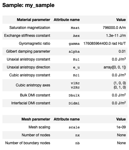
Any of the listed parameters can easily be changed using

sample.Msat = 796e3
sample.Aex = 13e-12
sample.alpha = 0.007
sample.scale = 10e-9

The uniaxial anisotropy can be defined to be homogeneous over the whole sample or to be spatially varying, both in magnitude and direction. The direction doesn’t need to be a unit vector and will not be normalized in the code. Therefore, the implementation allows to define directions in units of the anisotropy and set the anisotropy constant to 1. For details please check the next sections.

3.4.1.1. Homogeneous uniaxal anisotropy

A homogeneous uniaxial anisotropy can be set using a triplet for the direction and a single constant. For a single crystal ferromagnetic sample would be like:

sample.Ku = 48e3 # in J/m^3
sample.e_u = [1, 0, 0] # along the x axis

Easy plane anisotropies can also be defined, by setting the anisotropy constant to negative value. An example for an xy easy plane would be:

sample.Ku = -20e3 # in J/m^3
sample.e_u = [0, 0, 1] # along the z axis

3.4.1.2. Spatial-dependent uniaxal anisotropy

A spatial dependent uniaxial anisotropy can be defined by a list of triplets defining the orientation at each node position and by a list of the constants. The template vectorfields in tetrax.vectorfield can be used to define spatial dependent vectorfields.

Here is an example for a radial uniaxial anisotropy with a homogeneous anisotropy constant:

sample.Ku1 = 2e4 #J/m^3
sample.e_u = tx.vectorfields.radial(sample.xyz,1)

The defined vectorfield of the uniaxial anisotropy can be visualized to check if the aimed spatial dependence has been set or not. This can be done by the plot() method. For further details please check the provided example: Spatially dependent uniaxial anisotropy.

3.4.2. Antiferromagnetic samples

To be implemented.