Getting started

Installation

Install this package using

pip install git+https://gitlab.hzdr.de/micromagnetic-modeling/tetrax.git

To allow for 3D visualization in Jupyter notebooks, you additionally need to activate the k3d extension in your shell using

$ jupyter nbextension install --py --sys-prefix k3d
$ jupyter nbextension enable --py --sys-prefix k3d

Now you are ready to use TetraX in your python scripts or Jupyter notebook.

import tetrax as tx

For details, see User Guide: Installation.

Create a sample

The micromagnetic workflows in TetraX are centered around two main objects: The sample and the experimental setup. A sample mainly consists of a geometry, a set of material parameters and a magnetization vector field. An experimental setup is created around such a sample and consists of a fixed set of external parameters or objects, such as external magnetic field or microwave antennae.

To create a sample, we can choose from three different geometries (“confined”, “waveguide”, “layer”) and two different magnetic orders (“FM”/ferromagnetic or “AFM”/antiferromagnetic).

Note

As of version 1.3.0, only ferromagnetic waveguides and multilayers are fully supported, while antiferromagnets and confined samples (without dipolar interaction) are included as experimental features.

sample = tx.create_sample("my_sample")

# is the same as:
# sample = tx.create_sample("my sample", geometry="waveguide", magnetic_order="FM")

When a ferromagnetic sample is created, it will be initialized with the material parameters of NiFe (permalloy). When working in a Jupyter notebook, we can have a look at these parameters using

>>> sample

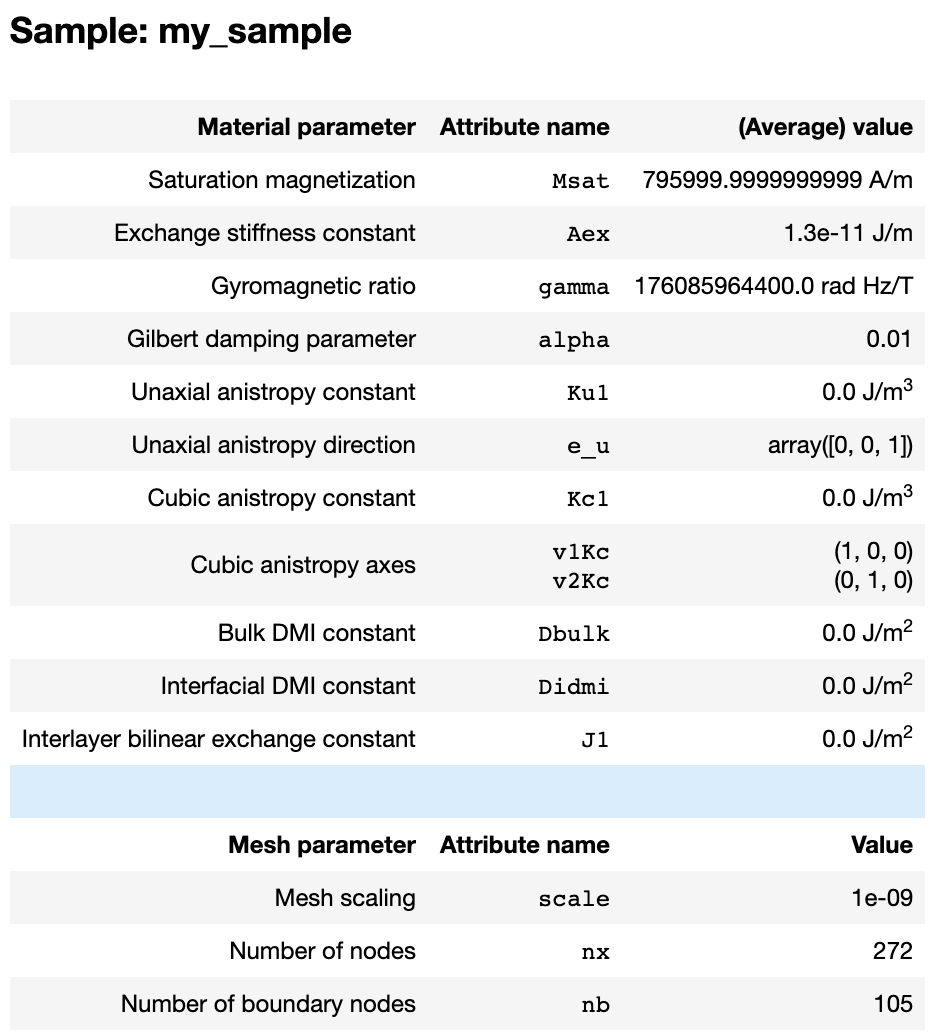
Any of these parameters can easily be changed using

sample.Msat = 796e3
sample.Aex = 13e-12

Notice that the third column shows the average values of each attribute, hinting at the fact that several of the material parameters can be spatially dependent (Msat, Aex and Ku1, see User Guide for details.). We can see at the bottom of the screenshot above, that the sample does not have a mesh yet. TetraX provides a number of predefined meshes which can be accessed from the tetrax.geometries submodule (see User Guide). There are several ways to assign a mesh to the sample. To show this, we let us create the cross section of a nanotube. Note, that all lengths within the mesh are scaled by the scale attribute of our sample object.

# Use a predefined mesh

r = 20     # inner radius
R = 30     # outer radius
lc = 3     # discretization of mesh

# sample.scale = 1e-9  ->  all mesh lengths are in nanometer

mesh = tx.geometries.tube_cross_section(r,R,lc=lc)

sample.set_geom(mesh)

# Define your own mesh using pygmsh

import pygmsh
with pygmsh.occ.Geometry() as geom:
    geom.characteristic_length_min = lc
    geom.characteristic_length_max = lc
    disk1 = geom.add_disk([0, 0.0], R)
    disk2 = geom.add_disk([0, 0.0], r)
    geom.boolean_difference(disk1,disk2)
    mesh = geom.generate_mesh()
    sample.set_geom(mesh)

# Read your own mesh from a file

sample.read_mesh("my_mesh.geo")

Once a mesh is set, we are able to inspect our mesh using

>>> sample.show()

We can see that sample.show() displays the two-dimensional mesh of the waveguide together with an extruded shaded volume that hints at the geometry of the full three-dimensional tube (this can be hidden with show_extrusion=False). Note, that meshes for waveguide cross sections need to be embedded in the \(xy\) plane, whereas meshes for layer samples need to be embedded on the \(y\) axis. Per default, a sample does not have a magnetization vector field yet. We can set it using

import numpy as np

sample.mag = np.array([1, 0, 0])
sample.show()

TetraX also provides a number of template vector fields in the tetrax.vectorfields submodule. For example, we can initialize our tube cross section in a helical state using

Theta = 60    # angle with z axis
chi = 1       # circularity

sample.mag = tx.vectorfields.helical(sample.xyz, 60, 1)
sample.show()

Run experiments

Setting up an experimental setup

In order to run numerical experiments, we need to place the same in a experimental setup.

exp = tx.create_experimental_setup(sample, name="Bphi_80mT")

The name parameter of the experimental setup is set to identify the data produced in our current setup. Now, all data produced by numerical experiments produced in this setup will be saved to the /my_sample/Bphi_80mT subdirectory of your working diretory. For our current example, we want to apply an azimuthal field (in \(\phi\) direction) of \(B_\phi = 80\,\mathrm{mT}\). For this, we can exploit the tetrax.vectorfields.helical() funtion used before.

B_phi = 0.08 # in Tesla

exp.Bext = B_phi * tx.vectorfields.helical(sample.xyz, 90, 1)
exp.show(scale=50,show_extrusion=False)

The experimental setup can also contain a microwave antenna, for example, to calculate a microwave-power absorption. For this, see the example Absorption of a nanotube with antennae or the User Guide.

Calculate equilibrium state

Once the experimental setup is set up, we can calculate the equilibrium-magnetization state of our sample with the given material and external parameters.

>>> exp.relax(tol=1e-11)
Minimizing in using 'L-BFGS-B' (tolerance 1e-11) ...
Current energy length density: 3.325805580142271e-11 J/m  mx = 0.00  my = -0.01  mz = -0.00
Success!

>>> sample.show()

We see that the equilibrium state of the sample in this setup is indeed a vortex state.

Normal modes analysis

We can calculate the dispersion of the (here) propagating normal modes using our propagating wave eigensolver. Depending on the geometry and magnetic order, the corresponding eigensolver will automatically be selected. It returns the mode frequencies (here: dispersion) as a DataFrame and saves the spatial (here: lateral) mode profiles as vtk files to the mode-profiles/ directory in the directory of the experimental setup.

dispersion = exp.eigenmodes(num_cpus=-1,num_modes=10)

Here, the num_cpus argument tells to use all available CPU cores for calculation. For further details, see User Guide.

We can plot the obtained dispersion easily using matplotlib.

%matplotlib notebook
import matplotlib.pyplot as plt
import matplotlib as mpl

for i in range(9):
   plt.plot(dispersion["k (rad/m)"]*1e-6, dispersion[f"f{i} (GHz)"])

plt.xlabel("k (rad/µm)")
plt.ylabel("f (GHz)")
plt.show()

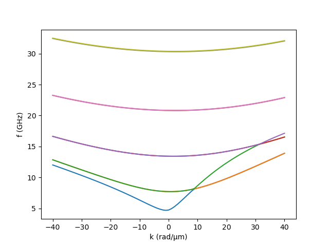
As seen, we have recovered the asymmetric spin-wave dispersion in a vortex-state magnetic nanotube. 1 The mode profiles can be visualized, for example, using ParaView. A built-in method to visualize mode profiles will be implemented in the future.

Run as a script

Of course, you can also run TetraX experiments in Python scripts (e.g. my_simulation.py), for example, to deploy them on a cluster. For this, it is important to add if __name__ == ‘__main__’ to the beginning of your script, otherwise the multiprocessing will overflow your memory and your script will crash. A valid script will look like this:

if __name__ == ‘__main__’:

   import tetrax as tx

   sample = tx.create_sample()
   ...

Where to go from here

For other useful examples, for example, how to calculate a microwave absorption, check out our Examples section or take a look into the User Guide.

References

1

Otálora, et al., “Curvature-Induced Asymmetric Spin-Wave Dispersion”, Phys. Rev. Lett. 117, 227203 (2016)