Double layers of Py / CoFeB#
example taken from the paper of Grassi et al., PHYSICAL REVIEW APPLIED 14, 024047 (2020)
[1]:
%matplotlib notebook
import matplotlib.pyplot as plt
import tetrax as tx
import numpy as np
Sample definition as one layer with inhom material parameters#
[2]:
dlayer_50 = tx.create_sample(geometry="layer",name="Py25CoFeB25")
t1_Py = 25
t2_CoFeB = 25
total_thickness = t1_Py + t2_CoFeB
res = 2.0
dlayer_50.set_geom(tx.geometries.monolayer_line_trace(total_thickness,res))
Setting geometry and calculating discretized differential operators on mesh.
Done.
Let’s define material parameters for the Py and CoFeB layers:
[3]:
dlayer_50.gamma = 29.2 * 2 * np.pi * 1e9

Msat_Py = 845e3
Msat_CoFeB = 1270e3
middle = -(total_thickness)/2 + t1_Py
Msat_ = np.piecewise(dlayer_50.xyz.x, [dlayer_50.xyz.y <= middle, dlayer_50.xyz.y > middle], [Msat_Py,Msat_CoFeB])
dlayer_50.Msat = Msat_

A_Py = 12.8e-12
A_CoFeB = 17e-12
Aex_ = np.piecewise(dlayer_50.xyz.x, [dlayer_50.xyz.y <= middle, dlayer_50.xyz.y > middle], [A_Py,A_CoFeB])
dlayer_50.Aex = Aex_

print("Msat_avrg=", dlayer_50.Msat_avrg)
print("gamma", dlayer_50.gamma)
Msat_avrg= 1057500.0
gamma 183469010969.6439
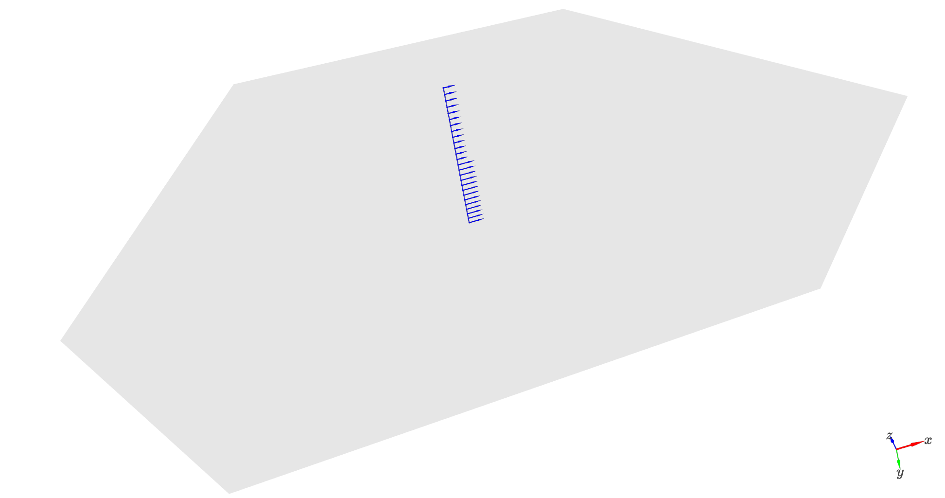
Setting parallel magnetization in the layers, depending on the thickness coordinates (y) and showing the sample:
[4]:
dlayer_50.mag = np.piecewise(dlayer_50.xyz, [dlayer_50.xyz.y <= middle, dlayer_50.xyz.y > middle], [[1,0,0],[1,0,0]])
dlayer_50.show()
/Users/attilak/anaconda3/lib/python3.10/site-packages/traittypes/traittypes.py:97: UserWarning: Given trait value dtype "float32" does not match required type "float32". A coerced copy has been created.
  warnings.warn(
Experiment with external field only#
relaxation of the state in a small external field
[5]:
exp = tx.create_experimental_setup(dlayer_50)
exp.Bext = [30e-3,0,0]
exp.relax()
dlayer_50.show()
Minimizing in using 'L-BFGS-B' (tolerance 1e-12) ...
Current energy length density: -2.297660589509063e-24 J/m  mx = 1.00  my = -0.00  mz = -0.00
Success!
Dispersion calculation for the first N=5 number of nodes#
[6]:
disp = exp.eigenmodes(kmin=-50e6,kmax=50e6,Nk=81, num_cpus=-1,num_modes=5,save_modes=True,no_dip=False)
100%|█████████████████████████████| 81/81 [00:12<00:00, 6.53it/s]
Plotting the dispersion#
[7]:
plt.rcParams["figure.figsize"] = (8,6)
plt.figure()

for i in range(2):
    plt.plot(disp["k (rad/m)"].values*1e-6,disp[f"f{i} (GHz)"].values,ls='--', linewidth=3, alpha=1)

plt.xlabel("wave vector (rad/µm)")
plt.ylabel("frequency (GHz)")
plt.xlim([-50,50])
plt.ylim([4,26])
plt.grid(color='0.95')
plt.show()
