Spatially dependent uniaxial anisotropy#
In this notebook we show how to set a spatially varying uniaxial anisotropy. To demonstrate we will use a nanotube (R=30 nm outer radius,r=20 nm inner radius) and set a radial uniaxial anisotropy.
[1]:
import tetrax as tx

%matplotlib notebook
import matplotlib.pyplot as plt
[2]:
sample = tx.create_sample(name="Nanotube_20nm_30nm")
sample.Msat = 800e3
sample.Aex = 13e-12
mesh = tx.geometries.tube_cross_section(20,30,lc=3)
sample.set_geom(mesh)
Setting geometry and calculating discretized differential operators on mesh.
Done.
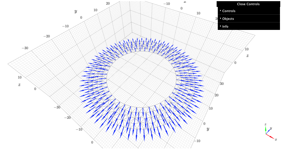
In the following we set a radial uniaxial anisotropy using the tx.vectorfields.radial(sample.xyz,1) function:
[3]:
sample.Ku1 = 2e4 #J/m^3
sample.e_u = tx.vectorfields.radial(sample.xyz,1)
sample.plot(sample.e_u)
[4]:
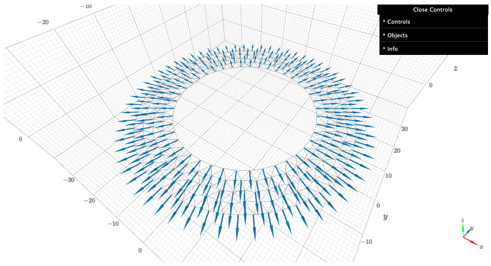
sample.mag = tx.vectorfields.radial(sample.xyz,1)
exp = tx.create_experimental_setup(sample)
exp.relax(tol=1e-9,continue_with_least_squares=True)
Minimizing in using 'L-BFGS-B' (tolerance 1e-09) ...
Current energy length density: 6.316798137122507e-10 J/m  mx = -0.01  my = -0.00  mz = 0.00
Relaxation with L-BFGS-B method was not succesful.

Minimizing in using SLSQP method (tolerance 1e-09) ...
Current energy length density: 6.316832551337032e-10 J/m  mx = -0.01  my = -0.00  mz = 0.000
Success!
[5]:
sample.show()