5. Visualization and evaluation

This chapter provides documentation on how to visualize and evaluate data.

5.1. Sample and experimental setup visualization

At the moment, samples and experimental setups can be inspected with

>>> sample.show()
>>> exp.show()

which will display a 3D view using the k3d package.

5.2. Scalar- and vectorfield visualization

It is also possible to plot scalar fields or vector fields defined on a given sample using the plot() method of a sample.

>>> vector_field = tx.vectorfields.helical(sample.xyz, 90, 1)
>>> sample.plot(vector_field)

5.3. Mode visualization

The calculated modes can be shown in the notebook using the show_mode(). The mode will be visualized as a vectorfield colored according to its magnitute, dark and bright colors represent low and high amplitudes, respectively. The mode can be visualized as the dynamic component only or as a mode on the top of the equilibrium magnetization.

The mode can be visualized with the following command:

>>> exp.show_mode(k=10,N=1,periods=10,on_equilibrium=True,animated=True,scale=10,fps=30,scale_mode=2)

This will show the animated mode movie of the mode N=1 for k=10 rad/µm wave vector, on the top of the equilibrium, for 10 periods with 30 frames per second. The magnetization vectorfield can be scaled by the scale parameter and the amplitude of the dynamic component with the scale_mode parameter.

Here is an example for a magnetostatic surface wave in a 50 nm permalloy film in the Damon-Eshbach geometry.

For details of the mode animation check the method:

5.4. Average and data extraction

In order to calculate the average of a given vector or scalar field on a sample, one can use the average() method of the respective sample.

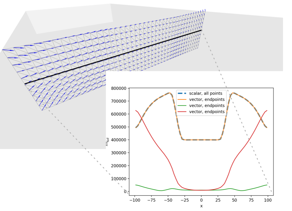
Extracting data of vector or scalar fields along a line or curve is possible with the scan_along_curve() method of the sample.