4. Numerical Experiments

4.1. The ExperimentalSetup object

4.1.1. Creating a setup and conducting experiments

The central object to conduct numerical experiments is the ExperimentalSetup class which is always associated to a sample. It can be created using

exp = tetrax.create_experimental_setup(sample, name="my_experiment")

As with the names of sample objects, the name attribute of the setup is only for saving purposes and is used to create directories for data calculated in numerical experiments. Within the setup, experimental conditions can be specified:

• Bext, a static external magnetic field given in units of Tesla, which, like the magnetization of the sample, is a MeshVector object (an array of shape (nx, 3)) for which template vectorfields are found in the tetrax.vectorfields module. Homogenous external fields can also be set for examples as

  exp.Bext = [0, 0, 5e-3]
  

• antenna is the microwave antenna in the experimental setup for which the microwave absorption of the spin-wave modes in the sample can be calculated, or which (in confined samples) can be used to apply time-dependent external fields. An antenna can be set using

  exp.antenna = tetrax.core.experimental_setup.CPWAntenna(150, 30, 54)
  

The full experimental setup, including external field and microwave antenna, can be visualized using

exp.show()

Within the setup, a number of numerical experiments can be conducted (which are documented below) as

exp.relax()
exp.eigenmodes()
exp.absorption()
exp.evolve() # only for confined samples

4.1.2. Microwave antennae

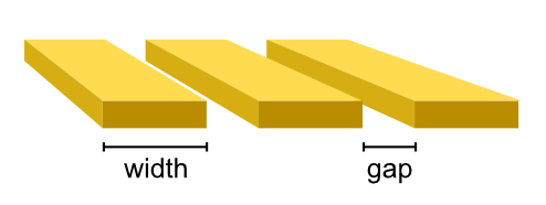
The available microwave antennae, called from the tetrax.core.experimental_setup module, are

class tetrax.core.experimental_setup.CPWAntenna(width, gap, spacing)

Coplanar-waveguide antenna. The antenna is assumed to be infinitely thin.

Attributes

widthfloat

Width of the current lines (in propagation direction).

gapfloat

Gap (not pitch) between the current lines.

spacingfloat

Distance between coordiante origin and antenna center plane.

Methods

get_mesh
get_microwave_field_function

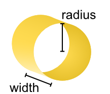
class tetrax.core.experimental_setup.CurrentLoopAntenna(width, radius)

Antenna with the shape of a current loop.

The current loop is oriented in the \(xy\) plane. For calculations, the current loop is taken to be infinitely thin in radial direction.

Attributes

widthfloat

Width of the antenna (in propagation direction).

radiusfloat

Radius of the antenna.

Methods

get_mesh
get_microwave_field_function

class tetrax.core.experimental_setup.HomogeneousAntenna(theta=0, phi=0)

Antenna which produces a homogeneous microwave field.

Attributes

thetafloat

Polar angle of the field polarization (given in degrees).

phifloat

Azimuthal angle of the field polarization (given in degrees).

Methods

get_mesh
get_microwave_field_function

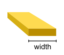
class tetrax.core.experimental_setup.StriplineAntenna(width, spacing)

Stripline antenna. The antenna is assumed to be infinitely thin.

Attributes

widthfloat

Width of the current lines (in propagation direction).

gapfloat

Gap (not pitch) between the current lines.

spacingfloat

Distance between coordiante origin and antenna center plane.

Methods

get_mesh
get_microwave_field_function

4.2. Energy minimization

For many purposes it is important to calculate the magnetic equilibrium state of a sample under given external conditions. There are many different ways to do this, with the simplest one being minimizing the total magnetic energy (the energy length density for waveguide samples and the energy area density for layer samples).

Warning

The relaxation in waveguide samples is not always stable and should be conducted with care.

After initializing the magnetization of the sample (mag) can be done using the relax() method.

tetrax.core.experimental_setup.ExperimentalSetup.relax(self, tol=1e-12, continue_with_least_squares=False, return_last=False, save_mag=True, fname='mag.vtk', verbose=True)

Relax the magnetization mag of a sample in the experimental setup by minimizing the total magnetic energy.

Parameters

tolfloat, optional

Tolerance at which the minimization is considered successful (default is 1e-12).

continue_with_least_squaresbool

If minimization with conjugate-gradient method was not successful, continue with least-squares method (default is False). This is more stable, but slower.

return_lastbool

If minimization was not successful, set the last iteration step as the sample magnetization (default is False).

save_magbool

Save the resulting magnetization as vtk file to the folder of the experimental setup (default is True).

fnamestr

Filename for magnetization file (default is mag.vtk).

verbosebool

Output progress of the calculation (default is True).

Returns

successbool

If the relaxation was successful of not.

Notes

For waveguide samples, the equilibration is not totally stable yet. Please use with care and check the resulting equilibrium states.

Examples

• Spin-wave dispersion in transversally-magnetized rectangular waveguide

• Hysteresis loop calculation

• Spatially dependent uniaxial anisotropy

4.3. Linear magnetization dynamics

4.3.1. Spin-wave normal-mode analysis

4.3.1.1. Mode frequencies (dispersion) and spatial profiles

To obtain the frequencies and spatial mode profiles of the spin-wave normal modes in a given sample, the linearized lossless Landau-Lifshitz-Gilbert equation

(1)\[ \frac{\omega_\nu}{\omega_M} \mathbf{m}_\nu = i [\mathbf{m}_0 \times \hat{\mathbf{\Omega}}]\mathbf{m}_\nu \quad \text{with} \quad \mathbf{m}_0 \perp \mathbf{m}_\nu\]

can be solved numerically using a dynamic-matrix approach. Here, \(\mathbf{m}_\nu\) are the complex-valued spatial profiles of the normal modes, \(\mathbf{m}_0\) is the normalized equilibrium magnetization, \(\omega_M = \mu_0\gamma M_\mathrm{s}\) is the characteristic frequency of the material and the operator \(\hat{\mathbf{\Omega}}\) is given as

\[\hat{\mathbf{\Omega}} = h_0 \hat{\mathbf{\Omega}} + \hat{\mathbf{N}}\]

with the projection of the (unitless) equilibrium effective field onto the equilibrium magnetization

\[h_0 = \mathbf{m}_0 \cdot (\mathbf{h}_\mathrm{ext} + \hat{\mathbf{N}}\mathbf{m}_0 ).\]

The operator \(\hat{\mathbf{N}}\) is a certain Hermetian operator, which contains the mangetic self interactions

\[\hat{\mathbf{N}} = \hat{\mathbf{N}}^\mathrm{(exc)} + \hat{\mathbf{N}}^\mathrm{(dip)} + \hat{\mathbf{N}}^\mathrm{(uni)} + \hat{\mathbf{N}}^\mathrm{(cub)} + \hat{\mathbf{N}}^\mathrm{(iDMI)} + \hat{\mathbf{N}}^\mathrm{(bDMI)}\]

and which we refer to here as the magnetic tensor. Its application to the magnetization yields the effective field. For the cubic anisotropy, a linearized operator is used, except for the equilibrium field \(h_0\) for which the full nonlinear field is used. For details, about the individual terms and their implementation, refer to the Micromagnetic model and implementation section in the appendix.

To implement the constraint \(\mathbf{m}_0 \perp \mathbf{m}_\nu\), the eigenvalue problem (1) is projected into the subspace locally orthogonal to the equilibrium direction \(\mathbf{m}_0\).

For propagating spin waves in waveguide, or layer samples, the eigenvalue problem is projected into a single cross section of the sample by making the replacements

\[\begin{split}\mathbf{m}_\nu \rightarrow \mathbf{m}_{\nu k} = \mathbf{m}_{\nu} e^{-ikz} \\ \hat{\mathbf{N}} \rightarrow \hat{\mathbf{N}}_k = e^{-ikz}\hat{\mathbf{N}} e^{ikz}\end{split}\]

with the wave vector in \(z\) direction \(k\), the lateral mode profiles \(\mathbf{m}_{\nu k}\) and the propagating-wave tensors \(\hat{\mathbf{N}}_k\). The eigenvalue problem is then solved for the lateral profiles and the dispersion \(\omega_\nu(k)\). For of the propagating-wave dynamic-matrix approach used here, see Ref 1.

Note

During the course of this User Guide, volumentric \(\mathbf{m}_\nu\) and lateral profiles \(\mathbf{m}_{\nu k}\) are often interchangeably denoted simply as “mode profiles”, unless stated otherwise.

In TetraX, the eigensystem of a given sample in an experimental setup exp can be calculated by

>>> dispersion = exp.eigenmodes(...)

or simply

>>> exp.eigenmodes(...)

By default, the oscillation frequencies and the mode profiles are saved into the directory of the experimental setup.

tetrax.core.experimental_setup.ExperimentalSetup.eigenmodes(self, kmin=- 40000000.0, kmax=40000000.0, Nk=81, num_modes=20, k=None, no_dip=False, h0_dip=False, num_cpus=1, save_modes=True, save_local=False, save_magphase=False, linewidths=False, perturbed_dispersion=False, save_stiffness_fields=False, verbose=True, save_disp=True, fname=None)

Calculate the spin-wave eigenmodes and their frequencies/dispersion of the sample in its current state using a dynamic matrix approach.

The eigensystem is calculuated by numerically solving the linearized equation of motion of magnetizion (see User Guide for details). For waveguides or layer samples, a finite-element propagating-wave dynamic-matrix approach is used [1]. The dispersion is returned as a pandas.DataFrame. Additionally, it is saved as dispersion.csv (or dispersion_perturbedmodes.csv, if perturbed_dispersion=True) in the folder of the experimental setup.

Parameters

kminfloat

Minimum wave vector in rad/m (default is -40e6). This argument is ignored when calculating the eigensystem for confined samples.

kmaxfloat

Maximum wave vector in rad/m (default is 40e6). This argument is ignored when calculating the eigensystem for confined samples.

Nkint

Number of wave-vector values, for which the mode frequencies are calculated. This argument is ignored when calculating the eigensystem for confined samples (default is 81).

num_modesint

Determines how many modes (for confined samples) or branches of the dispersion (for waveguides and layers samples) are calculated in total (default is 20).

kfloat or array_like

By supplying an array_like of wave vectors arbitrary k vector resolution is possible for particular or interesting parts of the dispersion. If set to a single float value, the eigensystem is only calculated for a single wave vector (default is None). This argument is ignored when calculating the eigensystem for confined samples.

no_dipbool

Exclude dipolar interaction from calculations (default is False).

h0_dipbool

If no_dip is True, still retain dipolar contributions in the equilibrium effective field.

num_cpusint

Number of CPU cores to be used in parallel for calculations (default is 1). If set to -1, all available cores are used.

save_modesbool

Saves real and imaginary part of the mode profiles in cartesian basis as vtk files (default is True). The mode profiles are saved in a /mode-profiles subdirectory in the folder of the experimental setup.

save_localbool

If save_modes is also True, save the components of the mode profiles in the basis locally orthogonal to the equilibrum magnitization (default is False). The local components are saved in the same vtk file as cartesian components.

save_magphasebool

If save_modes is also True, save magnetide and phase of the mode-profile components (default is False). Saved in the same

linewidthsbool

Calculates the linewidths \(\Gamma=\alpha\epsilon\omega\) of the modes (with precession ellipticities \(\epsilon\)) and adds \(\Gamma/2\pi\) in GHz to the dataframe (default is False).

perturbed_dispersionbool

After calculating the eigenmodes/normalmodes (possibly with no_dip=True), calculate the zeroth-order pertubation of the dispersion including dynamic dipolar fields according to Ref [2]. Gives approximation for dispersion without dipolar hybridization (default is False). The results are appended to the returned dispersion dataframe.

save_stiffness_fieldsbool

If perturbed_dispersion is also True, append the unitless individual stiffness fields (components) within the perturbed dispersion to the dispersion dataframe (default is False). Allows to numerically reverse engineer general spin-wave dispersions [2].

verbosebool

Output progress of the calculation (default is True).

save_dispbool

Save the computed dispersion to a csv file in directory of the experimental setup (default is True).

fnamestr

Filename for the dispersion file (default is "dispersion.csv" or dispersion_perturbedmodes, depending on perturbed_dispersion).

Returns

dispersionpandas.DataFrame

Dataframe (table) containing the calculated dispersion.

Notes

By default, the dispersion DataFrame is structured as

k (rad/m)	f0 (GHz)	f1 (GHz)	…
-40e6	1.426	2.352	…
…	…	…	…

In case linewidths=True, the linewidths are added in units of GHz as

k (rad/m)	f0 (GHz)	Gamma0/2pi (GHz)	…
-40e6	1.426	0.122	…
…	…	…	…

In case perturbed_dispersion=True, additional columns are added as

k (rad/m)	f0 (GHz)	f_pert_0 (GHz)	…
-40e6	1.426	484	…
…	…	…	…

Additionally, if save_stiffnessfields=True, the unitless stiffness fields per magnetic interaction are also appended

k (rad/m)	f0 (GHz)	f_pert_0 (GHz)	Re(N21_exc)_0	…
-40e6	1.426	484	0.431	…
…	…	…	…	…

Indivual columns/rows can be obtained in the usual way for pandas.DataFrame`, for example, with

>>> k = dispersion["k (rad/m)"]
>>> first_row = dispersion.iloc[0]

References

1

Körber, et al., “Finite-element dynamic-matrix approach for spin-wave dispersions in magnonic waveguides with arbitrary cross section”, AIP Advances 11, 095006 (2021)

2(1,2)

Körber and Kákay, “Numerical reverse engineering of general spin-wave dispersions: Bridge between numerics and analytics using a dynamic-matrix approach”, Phys. Rev. B 104, 174414 (2021)

Examples

• Spin-wave dispersion in thin vortex-state nanotube

• Spin-wave dispersion in transversally-magnetized rectangular waveguide

4.3.1.2. Linear mode damping

The linewidths \(\Gamma_\nu\) of the calculated normal modes can be calculated from the mode profiles and frequencies according to

\[\Gamma_\nu = \alpha_\mathrm{G} \epsilon_\nu \omega_\nu\]

with \(\alpha_\mathrm{G}\) being the Gilbert-damping parameter and \(\epsilon_\nu\) being the ellipticity coefficient of the respective mode which is calculated from the mode profile \(\mathbf{m}_\nu\) according to

\[\epsilon_\nu = -i\frac{\langle\vert\mathbf{m}_\nu\vert^2\rangle_\mathrm{S}}{\langle \mathbf{m}_\nu^* \cdot \mathbf{m}_0\times\mathbf{m}_\nu\rangle_\mathrm{S}}\]

with the equilibrium-magnetization direction \(\mathbf{m}_0\) and the sample average \(\langle ... \rangle_\mathrm{S}\) (see Ref 2 for spin waves in general samples and Ref 3 for propagating waves in waveguide samples). The linewidths can be automatically calculated together with the dispersion by setting linewidths=True when calling the eigenmodes() method, or, alternatively, using the linewidths() method.

tetrax.core.experimental_setup.ExperimentalSetup.linewidths(self, auto_eigenmodes=False, k=None, verbose=True, **kwargs)

Calculates the linewidths \(\Gamma=\alpha\epsilon\omega\) of spin-wave modes (with precession ellipticities \(\epsilon\)).

Parameters

auto_eigenmodesbool

If no modes have been previously calculated, calculates them automically (default is False).

kfloat

Wave number at which the linewidths should be calculated. If None, the full wave-vector range available from the dispersion will be used (default is None).

verbosebool

Output progress of the calculation (default is True).

kwargs

Optional keyword arguments to be passed to the eigensolver (e.g. num_cpus=-1).

Returns

linewidthspandas.DataFrame

Dataframe (table) containing the calculated linewidths (and the dispersion).

Notes

The line widths are returned together with the oscillation frequencies in units of GHz.

k (rad/m)	f0 (GHz)	Gamma0/2pi (GHz)	…
-40e6	1.426	0.122	…
…	…	…	…

References

1

Verba, et al., “Damping of linear spin-wave modes in magnetic nanostructures: Local, nonlocal, and coordinate-dependent damping”, Phys. Rev. B 98, 104408 (2018)

2

Körber, et al., “Symmetry and curvature effects on spin waves in vortex-state hexagonal nanotubes”, Phys. Rev. B 104, 184429 (2021)

Examples

• Dispersion and linewidths in thick film

4.3.1.3. Microwave absorption and dynamic susceptibility

If the experimental setup has an antenna, the high-frequency power absorption (microwave absorption) of the spin-wave normal modes can be calculated with respect to this antenna, as a function of frequency and wave vector (only for propagating waves).

The wave-vector- and frequency-dependent microwave absorption \(P(k,\omega)\) is calculated according to

\[P(k,\omega) \propto \sum\limits_\nu \frac{\vert h_\nu(k)\vert^2}{[\omega_\nu(k) - \omega]^2-\Gamma_\nu^2(k)}\]

where the index \(\nu\) runs over all calculated modes (per wave vector), \(\omega_\nu(k)\) are the mode angular frequencies and \(\Gamma_\nu(k) = \alpha_\mathrm{G}\epsilon_\nu(k)\omega_\nu(k)\) are the linewiths, determined from the Gilbert damping parameter \(\alpha_\mathrm{G}\) and the mode ellipticites (see previous section). The factor \(h_\nu(k)\) is given by the overlap of the microwave field distribution (possible wave-vector dependent) with the respective mode profile

\[h_\nu(k) = -i\frac{\langle\mathbf{m}_\nu^* \cdot \mathbf{h}(k)\rangle_\mathrm{S}}{\langle \mathbf{m}_\nu^* \cdot \mathbf{m}_0\times\mathbf{m}_\nu\rangle_\mathrm{S}}\]

with the equilibrium-magnetization direction \(\mathbf{m}_0\) and the sample average \(\langle ... \rangle_\mathrm{S}\) (see, for example, Appendix A of Ref 3 for details).

Note

Naturally, for confined samples, the \(k\) dependence of an antenna is exchanged by a \(z\) dependence.

In TetraX, the microwave absorption of a given sample in an experimental setup exp can be calculated by

>>> (absorbed_power, wave_vectors, frequencies) = exp.absorption(...)

or, for a single wave vector

>>> subsceptibility = exp.absorption(k=0, ...)

tetrax.core.experimental_setup.ExperimentalSetup.absorption(self, auto_eigenmodes=False, fmin=0, fmax=30, Nf=200, k=None, verbose=True)

Obtain the microwave absorption of the calculated eigensystem with respect to the microwave antenna in the experimental setup.

Parameters

auto_eigenmodesbool

If no eigenmodes are available in this experimental setup, calculate eigenmodes with default settings.

fminfloat

Minimum microwave frequency in GHz for which the absorption line is calculated (default is 0).

fmaxfloat

Maximum microwave frequency in GHz for which the absorption line is calculated (default is 30).

Nfint

Number of microwave frequencies for which the absorption is calculated (default is 200).

kfloat

If set to a value, the absorption line is calculated only for a single wave vector (default is None). Also, the full dynamic susceptibility is saved to a dataframe. This argument is ignored in confined samples.

verbosebool

Output progress of the calculation (default is True).

Returns

susceptibilitypandas.DataFrame

Only if k is not None or sample is a confined sample. Contains frequency-dependent real and imaginary part as well as magnitude as phase and magnitude of the averaged dynamic susceptiblity.

(absorbed_power, wave_vectors, frequencies)(numpy.ndarray, numpy.ndarray, numpy.ndarray)

If k is None and sample is a waveguide or a layer sample. Saves the wave-vector and frequency- dependent microwave-power absorption (absorbed_power) together with the corresponding wave vectors and frequencies as a 2D arrays.

Notes

The return of a wave-vector-dependent absorption calculation can be plotted using matplotlib as

>>> absorbed_power, wave_vectors, frequencies = exp.absorption(...)
>>> import matplotlib.pyplot as plt
>>> plt.pcolormesh(wave_vectors, frequencies, absorbed_power)

References

1

Verba, et al., “Damping of linear spin-wave modes in magnetic nanostructures: Local, nonlocal, and coordinate-dependent damping”, Phys. Rev. B 98, 104408 (2018)

2

Körber, et al., “Symmetry and curvature effects on spin waves in vortex-state hexagonal nanotubes”, Phys. Rev. B 104, 184429 (2021)

Examples

• FMR in a rectangular waveguide

• Absorption of a nanotube with antennae

4.3.2. Perturbation analysis and reverse-engineering of analytical spin-wave dispersions

Within the eigenmodes(), TetraX also provides the possibility to perform disentangle dipole-dipole hybridized modes and to numerically reverse-engineer the stiffness fields within a spin-wave dispersion (see Ref. 4).

For example, the zeroth-order dipolar perturbation of exchange modes can be calculated using

>>> exp.absorption(..., no_dip=True, perturbed_dispersion=True)

This will first calculate the normal modes without dipolar interaction and then calculate their perturbed frequency including dynamic dipolar fields and neglecting hybridization. As stated in 4 only works well, if the spatial mode profiles are not changed considerably by the dipolar interaction. If desired, dipolar fields can still be included in the equilibrium field by supplying h0_dip=True.

During the calculation, the stiffness fields \(N_\nu^{(ij)}\) (\(i,j=1,2\)) within the general spin-wave dispersion

\[\frac{\omega_\nu(k)}{\omega_M} = \mathrm{Im}\, N_\nu^{(21)} + \sqrt{\Big(N_\nu^{(11)} + \langle h_0 \rangle_\mathrm{S} \Big)\Big(N_\nu^{(22)} + \langle h_0 \rangle_\mathrm{S} \Big) - \Big(\mathrm{Re}\, N_\nu^{(21)} \Big)^2}\]

are calculated for each mode and magnetic interaction 4.

They can be saved into the dispersion dataframe by supplying save_stiffness_fields=True. This method can of course also be used for the true dipole-exchange normal modes (no_dip=False) and allow, for example, to disentangle the contributions of different magnetic interactions to the magnetochiral stiffness field responsible for any dispersion asymmetry,

\[\mathrm{Im}\, N_\nu^{(21)} \equiv \mathcal{A}_\nu = \mathcal{A}_\nu^\mathrm{(dip)} + \mathcal{A}_\nu^\mathrm{(DMI)} + ...\]

For details of the calculations, we refer to Ref 4.

4.4. Nonlinear LLG dynamics

This feature will be implemented in a future release.

4.5. References

1

Körber, et al., “Finite-element dynamic-matrix approach for spin-wave dispersions in magnonic waveguides with arbitrary cross section”, AIP Advances 11, 095006 (2021)

2

Verba, et al., “Damping of linear spin-wave modes in magnetic nanostructures: Local, nonlocal, and coordinate-dependent damping”, Phys. Rev. B 98, 104408 (2018)

3(1,2)

Körber, et al., “Symmetry and curvature effects on spin waves in vortex-state hexagonal nanotubes”, Phys. Rev. B 104, 184429 (2021)

4(1,2,3,4)

Körber and Kákay, “Numerical reverse engineering of general spin-wave dispersions: Bridge between numerics and analytics using a dynamic-matrix approach”, Phys. Rev. B 104, 174414 (2021)